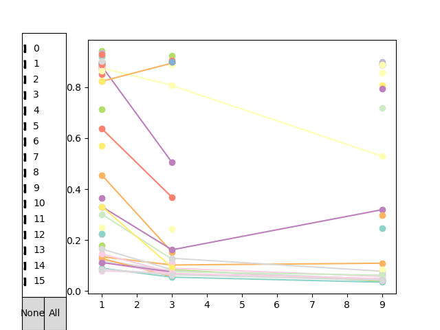
示例 7 - 结果的交互式探索

本示例使用示例 5 的一次运行结果，让您可以交互式地查看所有执行的运行及其相关的损失。图表允许您只包含某些迭代（通过左侧的复选框选择）。将鼠标悬停在学习曲线上（单个配置在所有相应预算下的所有运行），您会看到有关该配置及其性能的一些信息。点击曲线将使工具提示保持显示。再次点击曲线将移除工具提示。

此工具尚不成熟，但或许可以帮助您探索结果中隐藏的结构。请参阅可视化子模块的文档以查看所有选项。

• 
• 

import matplotlib.pyplot as plt
import hpbandster.core.result as hpres
import hpbandster.visualization as hpvis



# load the example run from the log files
result = hpres.logged_results_to_HBS_result('example_5_run/')

# get all executed runs
all_runs = result.get_all_runs()

# get the 'dict' that translates config ids to the actual configurations
id2conf = result.get_id2config_mapping()

lcs = result.get_learning_curves()

hpvis.interactive_HBS_plot(lcs, tool_tip_strings=hpvis.default_tool_tips(result, lcs))




def realtime_learning_curves(runs):
    """
    example how to extract a different kind of learning curve.

    The x values are now the time the runs finished, not the budget anymore.
    We no longer plot the validation loss on the y axis, but now the test accuracy.

    This is just to show how to get different information into the interactive plot.

    """
    sr = sorted(runs, key=lambda r: r.budget)
    lc = list(filter(lambda t: not t[1] is None, [(r.time_stamps['finished'], r.info['test accuracy']) for r in sr]))
    return([lc,])

lcs = result.get_learning_curves(lc_extractor=realtime_learning_curves)

hpvis.interactive_HBS_plot(lcs, tool_tip_strings=hpvis.default_tool_tips(result, lcs))

脚本总运行时间： ( 0 分钟 0.251 秒)